6  Aim 3 - Control of latent population dynamics

Rationale

As technology for recording from the brain has improved, systems neuroscience has shifted increasingly towards a reduced-dimensionality, population coding perspective in many brain areas (1–4). This reflects the observation that while the activity of any single neuron can vary greatly across trials where external variables are controlled, underlying latent variables can be decoded from the population which are much more predictable and reproducible. Moreover, formulating this latent variable as a dynamical state whose evolution can be predicted has been shown to improve inference and enable state-of-the-art “decoding” of downstream variables of interest such as movement (5–8), mood (9), speech (10), and decision states (11, 12). Not only does this allow us to infer the output of a given brain region, but it allows us to form hypotheses about how it produces that output by analyzing the dynamical landscape of fixed points (13–15)—a view formalized in the Computation through Dynamics (CTD) framework (16).

However, while these latent variables have been used to successfully decode other variables of interest, this is a necessary, but insufficent, condition to demonstrate a causal relationship. That is, an association between neural activity variable \(a\) and some other variable \(b\) may reflect the causal relationship \(a \rightarrow b\), but could also reflect \(b \rightarrow a\) or \(a \leftarrow c \rightarrow b\). This may be adequate for brain-computer interface (BCI) applications, but verification of that causal relationship is necessary for neuroscience’s goal of deepening our understanding of the architecture and algorithms of brain computations. This requires experimental control (17) on the level of neural populations, but, as stated by (16),

The challenge is nontrivial; testing CTD models requires a high degree of control over neural activity. The experimenter must be able to manipulate neural states arbitrarily in state space and then measure behavioral and neural consequences of such perturbations[.]

CLOC is a natural candidate for this kind of experimental control of latent states for various reasons. The optimal state-space methods already formulated map directly to the latent dynamics models which have generated so much interest in recent systems neuroscience. High-dimensional optogenetic actuation is possible through micro-LED devices (18–29), two-photon targeting of individual neurons (30–34), and genetic targeting. Moreover, real-time feedback can drive a variable neural system towards complex latent state targets which would be attainable with low accuracy at best and not at all at worst with open-loop stimulation ¹. However, while it is clear a high degree of control will be needed, it is unknown how this translates to recording, stimulation, and control parameters. One significant open question is whether this kind of control will require actuation on the level of individual neurons, or whether lower-dimensional actuation will suffice. I hypothesize that the latter is the case, but testing this hypothesis will likely require extensive trial and error, as well actuation hardware that does not exist or is not readily available, making it costly if not infeasible to do in vivo.

Innovation

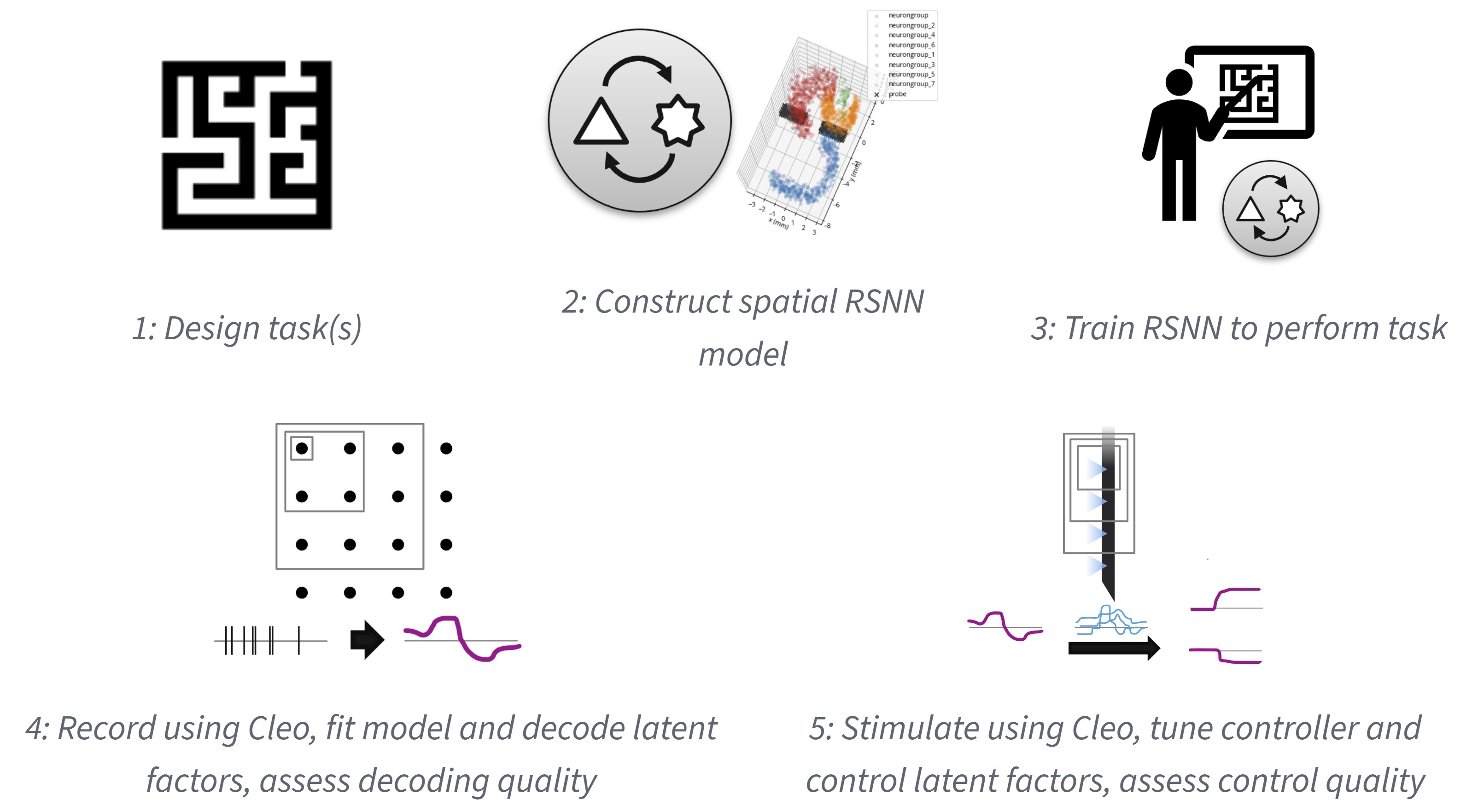
Thus, to give a preliminary answer to this question, I propose to develop technical and conceptual guidelines as I control the latent dynamics of simulated neural populations. First, I will produce virtual models by training recurrent spiking neural networks with state-of-the-art, biologically plausible methods—each differing in their degrees of brain-like architecture and training procedure complexity. I will then use the simulation testbed of Aim 1 and the multi-input control methods of Aim 2 to explore how control quality varies with both experimental parameters (such as recording and stimulation channel counts or control algorithms) and system characteristics (such as the size, complexity of the network model). This will both give researchers a tentative idea of the relative importance of each factor of CLOC and, as parameters approach experimental realism, allow us to conjecture as to the number of independent actuators needed to control the latent dynamics of a brain system. My hypothesis is that control quality will plateau with a number of actuators on or near the same level of magnitude as the latent factors used to describe the neural activity—that per-neuron actuation limit not be needed.

Approach

Figure 6.1: Overview of latent factor control experiments.

Formulate task with latent dynamics hypothesis

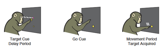
To model an experiment of interest to neuroscientists, I will first choose a task where latent dynamic analyses have yielded testable hypotheses in animal research. For example, it is hypothesized that motor cortex works as a dynamical system where movement planning essentially sets an initial condition during a preparatory phase. This is demonstrated specifically by decoding reach direction in a delayed reach task from dorsal premotor cortex before movement onset (35, reviewed in 36) (see Figure 6.2). One way to causally test this hypothesis would be to manipulate the latent factors corresponding to a certain reach direction despite an absent or contradictory cue and verify whether the subject reaches in the predicted direction.

Figure 6.2: Illustration of a delayed center-out reach experiment. From (37).

Train RSNN models

After identifying a task and latent dynamics hypothesis to test, I will train recurrent spiking neural network (RSNN) models to perform the task. These RSNN models will be defined in 3D space to make them compatible with the electrode and optogenetics models from Aim 1. To avoid painstaking implementation of every known anatomical detail of the brain region(s) involved in the task—an approach which is not guaranteed to include every important detail or capture true circuitry—I propose using a simple, abstract form such as a rectangular prism of cortical tissue and measuring the effect of adding progressivley more brain-like structural constraints (see Section 6.2.6).

I will then train these models to perform the given task. While a few different methods for training RSNNs exist, I plan on using e-prop (38), a biologically plausible approximation to backpropagation through time (BPTT), the method typically used to train artificial recurrent neural networks (RNNs). This biological plausibility consists in updating synaptic weights using only local information about past activity—“eligibility traces”—and a top-down learning signal and enables learning sparsely firing spike-coding—as opposed to only rate-coding—solutions. While e-prop has been shown to learn complex tasks such as Atari games via reinforcement learning, I propose a simpler supervised learning approach. This is both more data-efficient and would directly allow for the learning of auxiliary variables, which has been shown in one study to make model dynamics more brain-like (39) (see Section 6.4).

To give a concrete example of inputs and outputs for the case of the delayed center-out reaching task before mentioned, inputs might include the task phase (stop or go), the target position, and the current hand position. The model output might be hand velocity, and the learning signal could be computed from the x/y distance between the current position and the center (target) before (after) the go cue is given. A regularizer term on acceleration could be added to ensure trajectories are smooth.

Fit dynamical systems model

After a model has been trained to some threshold performance level, I will record spikes and/or LFP from the network while it performs the task. The resulting data will then be used to fit a low-dimensional dynamical systems model. Seeing that the goal of the virtual experiment is to test the causal effect of a latent factor on model output, I propose using system identification methods that prioritize the discovery of those latent factors that are most relevant to behavior. The preferential subspace identification (PSID) method presented by (7) is a good candidate, having been shown to predict behavior well with few dimensions. The linear system it produces is also ideal for the control theory methods I develop in Aim 2. In a follow-up study, (8) introduce RNN-PSID supporting nonlinearities as well and find empirically that linear dynamics with only a nonlinear mapping from latent to behavior are often sufficient to describe experimental data well. Using a potentially nonlinear output mapping in this way would increase the expressiveness of my models while maintaining underlying linear dynamics for fast optimization.

After fitting a model to data, I will identify latent factors corresponding to variables of interest. These could be individual components of the latent state \(x\) directly or simple (e.g., linear) transformations of \(x\). In the delayed center-out reaching task, for example, I would expect two factors with which the state at the end of the preparatory period can be used to predict the cued target position.

Control of latent factors

The next step is then to test whether these latent factors do in fact cause the behavior we observe. Importantly, the model and hypothesis from the previous step were formed without stimulation, since our stated goal is to causally test the latent factors we deduce from passive observation. Thus, I will first need to expand the model by simulating random optogenetic stimulation and fitting an input model—e.g., an input matrix \(B\) for the typical LDS case. If this is insufficient to fit the data well, I may need to increase the dimensionality of the latent state \(x\) to account for the actuator state (i.e., opsin kinetics) or dimensions of neural activity not arising during unperturbed activity.

With an input model, I will then be able to run control experiments. The methods from Aim 2 will calculate optimal actuation strategies as the simulation progresses to drive the identified latent factors to the desired state. Control quality will be assessed for each experiment using metrics such as mean-squared error (MSE) and will serve as the criterion for how successful the experiment was, seeing that low error serves the larger goal of testing the causal relationship with model behavior.

Exploration of experiment parameters and expected effects

To guide experimental design, I propose repeating the above process many times to explore how different factors affect control quality, thus informing which investments might be most fruitful. These factors might include:

• Control type. Open-loop control is faster and easier but cannot counteract variability inherent to the system and in the presence of model mismatch will fail to reach the target. Closed-loop methods will almost certainly perform better, but are harder to implement. Moreover, closed-loop control offers a range of options spanning the cost/quality spectrum, with the fast linear quadratic regulator (LQR) on one end and the expensive long-horizon, high-resolution model predictive control (MPC) on the other.
• Total recording/stimulation channel count (\(m + k\)). It may be helpful to think of these two parameters together, since they both require limited space in a device that is placed in or on the brain. I expect control quality to increase with channel count up to a point where the computational cost required for closed-loop control outweighs the benefits.
• Recording/stimulation channel ratio (\(m/k\)). Related to the previous point, when space for interface is hardware, it is an open question whether the current landscape of neuroscience technology, which has prioritized high-channel-count recording over stimulation, is the most effective for causal perturbations of neural dynamics.
• Data collection budget. Data collection is not free, and thus must be considered especially when considering the data-efficiency advantages of feedback control. This is also relevant for choosing models to control the system—with little training data, for example, a simple, easy-to-fit model may outperform a more expressive, data-hungry one.
• Optogenetic stimulation parameters. These could include the number and type of opsins and genetic targeting. Using at least two opsins could be expected to perform better than just one, as shown in Aim 2, though many more might not be useful due to overlapping spectral sensitivity and increased computation time. The effect of genetic targeting will likely depend on how well the targeted population correlates with the latent factor of interest.

Exploration of model realism and expected effects

As explained above, I propose using abstract RSNN models with varying degrees of brain-like realism rather than extremely detailed models. This is because highly detailed models are difficult to develop and expensive to simulate—moreover, it is hard to say exactly when a model has enough to detail to behave similarly to a real brain. On the other hand, by assessing the effect of a handful of brain-like features on how well we can contol latent neural dynamics in silico, I hope to identify trends that give a rough outlook of doing so in vivo. For example, if control quality tends to drop with the addition of each feature, we might infer control of a real brain will be considerably more challenging than in simulations. On the other hand, if control quality does not decrease considerably with brain similarity, we might have reason to be more optimistic.

The brain-like features I propose assessing include structural characteristics such as:

• Variability. Brains are far from deterministic, with unpredictability on the level of synaptic transmission all the way up to firing rates across a population. Small-scale stochasticity encourages redundance and robustness, which may make the model harder to “hack,” or perturb unnaturally. I expect that large-scale variability, such as an unmodeled input to the region, will highlight the advantages of feedback control.
• Network size (how many neurons are in the model). More neurons would likely mean more dimensions along which activity can vary, complicating the prospect of arbitrary control.
• Subpopulation structure. This could include constraining connectivity to circuits of brain regions, cortical layers, and cell types. This could also make control harder if the latent factor to control operates in cells that are multiple synapses away from those stimulated or if dynamics become driven by recurrent connections more than stimulation.
• Connectivity profiles. Cell pairs within a given population might have a uniform or a spatially dependent connection probability. I expect this, like subpopulation structure, to encourage segregated dynamics which could be either easier or harder to perturb.
• Cell diversity. Cells might have uniform or a random distribution of parameters such as membrane resistance, synaptic transmission delays, resting potentials, adaptivity, etc. Again, I expect this would encourage the segregation of neural dynamics.
• Neuron model complexity. Individual cell models could range from simple leaky integrate-and-fire (LIF) to Hodgkin-Huxley dynamics. I do not expect this to considerably impact control quality.

They also include characteristics about how the model is trained. A real brain regions is capable of performing not only one, simple, stereotyped task, but many tasks in many contexts. Therefore, another way to make models more brain-like is to diversify their experience—to train them on other tasks. It has been shown that this can result in an RNN reusing computational motifs learned in one task to solve others (40, 41).

Expected results

In addition to the specific expectations for experimental and model parameters described above, I expect that control quality will be relatively low (error will be high) especially for low actuator counts \(k\). However, as previously stated, I do not anticipate that \(k\) will need to approach the per-neuron limit either; rather, that low-error control will be possible with \(k\) close to the same order of magnitude as the latent state dimensionality. While expectations for each brain-like model feature are explained above, I predict that on the whole, control quality will decrease as models become more realistic. However, I predict that that that decrease will plateau, providing some confidence in my results and assurance that the complexity of the real brain may not be an insurmountable barrier to future in-vivo experiments.

Potential pitfalls & alternative strategies

One potential problem is that the RSNN models could learn dynamics that are not very brain-like. For example, they might learn a complicated feedforward function instead of tracking latent variables in a more natural way, in which case explicitly teaching the models to track variables of interest has been shown to make dynamics more brain-like (39). Alternatively, the latent variables decoded could be dominated by very few neurons, thus producing “latent variables” which are not actually latent and distributed, as in the brain. This can be avoided by regularizing the state inference step to discourage sparsity, thus inferring the state from a more diverse set of neurons.

Another caveat to generalizing conclusions is that the proposed perturbations may be unnatural—by perturbing the latent factors decoded from passive observation, I may unwittingly by pushing neurons “off-manifold,” causing them to fire in unnatural combinations (42). While it is beyond the scope of the proposed work to avoid this, I can at least quantify the phenomenon via the proxy of neural activity unexplained by our latent dynamical, assuming our intrinsic manifold is a subspace rather than a lower-dimensional attractor structure embedded therein (16, 43). For example, if under passive observation we can predict 95% of neural activity, and that drops to 50% under perturbation, we could conclude that 45% of the activity is now unnatural, as it must be explained by dimensions of activity introduced by stimulation.

Besides conceptual obstacles, the proposed work also has practical challenges, such as its large scale. To adequately assess control prospects across the whole space of experiment and structural factors described could represent a prohibitively high computational cost. This can be mitigated by avoiding a grid search of this space, analyzing random combinations of features or just one at a time rather than every single combination. Another factor in the computational cost is the speed of the training, model fitting, and control simulations themselves. In the case that simulations are too slow with the Brian/Cleo framework described in Aim 1, it may be worth exploring simpler simulations for the training step which does not require Cleo. This could involve using fast differential equation solvers (44) for the training step or even a less biological learning algorithm such as backpropagation through time with surrogate gradients for the nondifferentiable spike threshold function (45). Training might also be accelerated using a form of “warm start” where weights are initialized from a pre-trained model, though care would need to be taken that the effects of the warm start on learned dynamics not overshadow those of the structural features being tested.

Additionally, there is a possibility that RNN-PSID requires nonlinear terms to fit model data well, despite the authors’ findings that linear dynamics are often sufficient (8). In the case that nonlinearities preclude the formulation of MPC as a fast quadratic program, I may need to turn to neural networks, which, after training, could quickly produce approximate solutions for nonlinear optimization problems (see Section 5.5).

1.

J. F. Kalaska, R. Caminiti, A. P. Georgopoulos, Cortical mechanisms related to the direction of two-dimensional arm movements: Relations in parietal area 5 and comparison with motor cortex. Experimental Brain Research. 51, 247–260 (1983).

2.

M. M. Churchland, J. P. Cunningham, M. T. Kaufman, J. D. Foster, P. Nuyujukian, S. I. Ryu, K. V. Shenoy, K. V. Shenoy, Neural population dynamics during reaching. Nature. 487, 51–56 (2012).

3.

J. P. Cunningham, B. M. Yu, Dimensionality reduction for large-scale neural recordings. Nature neuroscience. 17, 1500–9 (2014).

4.

D. L. Barack, J. W. Krakauer, Two views on the cognitive brain. Nature Reviews Neuroscience. 22, 359–371 (2021).

5.

C. Pandarinath, D. J. O’Shea, J. Collins, R. Jozefowicz, S. D. Stavisky, J. C. Kao, E. M. Trautmann, M. T. Kaufman, S. I. Ryu, L. R. Hochberg, J. M. Henderson, K. V. Shenoy, L. F. Abbott, D. Sussillo, Inferring single-trial neural population dynamics using sequential auto-encoders. Nature Methods. 15, 805–815 (2018).

6.

F. R. Willett, D. T. Avansino, L. R. Hochberg, J. M. Henderson, K. V. Shenoy, High-performance brain-to-text communication via handwriting. Nature. 593, 249–254 (2021).

7.

O. G. Sani, H. Abbaspourazad, Y. T. Wong, B. Pesaran, M. M. Shanechi, Modeling behaviorally relevant neural dynamics enabled by preferential subspace identification. Nature Neuroscience. 24, 140–149 (2021).

8.

O. G. Sani, B. Pesaran, M. M. Shanechi, M. Hsieh, Where is all the nonlinearity: Flexible nonlinear modeling of behaviorally relevant neural dynamics using recurrent neural networks. bioRxiv, 2021.09.03.458628 (2021).

9.

O. G. Sani, Y. Yang, M. B. Lee, H. E. Dawes, E. F. Chang, M. M. Shanechi, Mood variations decoded from multi-site intracranial human brain activity. Nature Biotechnology. 36, 954–961 (2018).

10.

G. K. Anumanchipalli, J. Chartier, E. F. Chang, Speech synthesis from neural decoding of spoken sentences. Nature. 568, 493–498 (2019).

11.

A. S. Morcos, C. D. Harvey, History-dependent variability in population dynamics during evidence accumulation in cortex. Nature Neuroscience. 19, 1672–1681 (2016).

12.

T. D. Kim, T. Z. Luo, J. W. Pillow, C. D. Brody, "Inferring Latent Dynamics Underlying Neural Population Activity via Neural Differential Equations" in Proceedings of the 38th International Conference on Machine Learning (PMLR, 2021), pp. 5551–5561.

13.

D. Sussillo, O. Barak, Opening the Black Box: Low-Dimensional Dynamics in High-Dimensional Recurrent Neural Networks. Neural Computation. 25, 626–649 (2013).

14.

D. Sussillo, Neural circuits as computational dynamical systems. Current Opinion in Neurobiology. 25, 156–163 (2014).

15.

J. T. H. Smith, S. W. Linderman, D. Sussillo, "Reverse engineering recurrent neural networks with Jacobian switching linear dynamical systems" in Advances in Neural Information Processing Systems (2021; https://arxiv.org/abs/2111.01256), vol. 20, pp. 16700–16713.

16.

S. Vyas, M. D. Golub, D. Sussillo, K. V. Shenoy, Computation through Neural Population Dynamics. Annual Review of Neuroscience. 43, 249–275 (2020).

17.

J. Pearl, Causality (Cambridge University Press, New York, 2009).

18.

S. Dufour, Y. D. Koninck, Optrodes for combined optogenetics and electrophysiology in live animals. Neurophotonics. 2, 031205 (2015).

19.

K. Y. Kwon, H.-M. Lee, M. Ghovanloo, A. Weber, W. Li, Design, fabrication, and packaging of an integrated, wirelessly-powered optrode array for optogenetics application. Frontiers in Systems Neuroscience. 9 (2015).

20.

M. Welkenhuysen, L. Hoffman, Z. Luo, A. De Proft, C. Van den Haute, V. Baekelandt, Z. Debyser, G. Gielen, R. Puers, D. Braeken, An integrated multi-electrode-optrode array for in vitro optogenetics. Scientific Reports. 6, 20353 (2016).

21.

L. Wang, K. Huang, C. Zhong, L. Wang, Y. Lu, Fabrication and modification of implantable optrode arrays for in vivo optogenetic applications. Biophysics Reports. 4, 82–93 (2018).

22.

N. McAlinden, Y. Cheng, R. Scharf, E. Xie, E. Gu, C. F. Reiche, R. Sharma, P. Tathireddy, P. Tathireddy, L. Rieth, S. Blair, K. Mathieson, Multisite microLED optrode array for neural interfacing. Neurophotonics. 6, 035010 (2019).

23.

D. Mao, N. Li, Z. Xiong, Y. Sun, G. Xu, Single-Cell Optogenetic Control of Calcium Signaling with a High-Density Micro-LED Array. iScience. 21, 403–412 (2019).

24.

D. Mao, Z. Xiong, M. Donnelly, G. Xu, Brushing-Assisted Two-Color Quantum-Dot Micro-LED Array Towards Bi-Directional Optogenetics. IEEE Electron Device Letters. 42, 1504–1507 (2021).

25.

Y. Ohta, M. C. Guinto, T. Tokuda, M. Kawahara, M. Haruta, H. Takehara, H. Tashiro, K. Sasagawa, H. Onoe, R. Yamaguchi, Y. Koshimizu, K. Isa, T. Isa, K. Kobayashi, Y. M. Akay, M. Akay, J. Ohta, Micro-LED Array-Based Photo-Stimulation Devices for Optogenetics in Rat and Macaque Monkey Brains. IEEE Access. 9, 127937–127949 (2021).

26.

J. Antolik, Q. Sabatier, C. Galle, Y. Frégnac, R. Benosman, Assessment of optogenetically-driven strategies for prosthetic restoration of cortical vision in large-scale neural simulation of V1. Scientific Reports. 11, 1–18 (2021).

27.

S. Jeon, Y. Lee, D. Ryu, Y. K. Cho, Y. Lee, S. B. Jun, C.-H. Ji, Implantable Optrode Array for Optogenetic Modulation and Electrical Neural Recording. Micromachines. 12, 725 (2021).

28.

C. Kathe, F. Michoud, P. Schönle, A. Rowald, N. Brun, J. Ravier, I. Furfaro, V. Paggi, K. Kim, S. Soloukey, L. Asboth, T. H. Hutson, I. Jelescu, A. Philippides, N. Alwahab, J. Gandar, D. Huber, C. I. De Zeeuw, Q. Barraud, Q. Huang, S. P. Lacour, G. Courtine, Wireless closed-loop optogenetics across the entire dorsoventral spinal cord in mice. Nature Biotechnology. 40, 198–208 (2022).

29.

D. Eriksson, A. Schneider, A. Thirumalai, M. Alyahyay, B. de la Crompe, K. Sharma, P. Ruther, I. Diester, Multichannel optogenetics combined with laminar recordings for ultra-controlled neuronal interrogation. Nature Communications. 13, 985 (2022).

30.

A. M. Packer, L. E. Russell, H. W. P. Dalgleish, M. Häusser, Simultaneous all-optical manipulation and recording of neural circuit activity with cellular resolution in vivo. Nature Methods. 12, 140–146 (2015).

31.

E. Ronzitti, R. Conti, V. Zampini, D. Tanese, A. J. Foust, N. Klapoetke, E. S. Boyden, E. Papagiakoumou, V. Emiliani, Submillisecond Optogenetic Control of Neuronal Firing with Two-Photon Holographic Photoactivation of Chronos. Journal of Neuroscience. 37, 10679–10689 (2017).

32.

I.-W. Chen, E. Papagiakoumou, V. Emiliani, Towards circuit optogenetics. Current Opinion in Neurobiology. 50, 179–189 (2018).

33.

Z. Zhang, L. E. Russell, A. M. Packer, O. M. Gauld, M. Häusser, Closed-loop all-optical interrogation of neural circuits in vivo. Nature Methods. 15, 1037–1040 (2018).

34.

S. Sridharan, M. A. Gajowa, M. B. Ogando, U. K. Jagadisan, L. Abdeladim, M. Sadahiro, H. A. Bounds, W. D. Hendricks, T. S. Turney, I. Tayler, K. Gopakumar, I. A. Oldenburg, S. G. Brohawn, H. Adesnik, High-performance microbial opsins for spatially and temporally precise perturbations of large neuronal networks. Neuron. 110, 1139–1155.e6 (2022).

35.

M. M. Churchland, J. P. Cunningham, M. T. Kaufman, S. I. Ryu, K. V. Shenoy, Cortical Preparatory Activity: Representation of Movement or First Cog in a Dynamical Machine? Neuron. 68, 387–400 (2010).

36.

J. A. Gallego, M. G. Perich, L. E. Miller, S. A. Solla, Neural Manifolds for the Control of Movement. Neuron. 94, 978–984 (2017).

37.

G. Santhanam, B. M. Yu, V. Gilja, S. I. Ryu, A. Afshar, M. Sahani, K. V. Shenoy, Factor-Analysis Methods for Higher-Performance Neural Prostheses. Journal of Neurophysiology. 102, 1315–1330 (2009).

38.

G. Bellec, F. Scherr, A. Subramoney, E. Hajek, D. Salaj, R. Legenstein, W. Maass, A solution to the learning dilemma for recurrent networks of spiking neurons. Nature Communications. 11 (2020), doi:10.1101/738385.

39.

R. Rajalingham, A. Piccato, M. Jazayeri, Recurrent neural networks with explicit representation of dynamic latent variables can mimic behavioral patterns in a physical inference task. Nature Communications. 13, 1–15 (2022).

40.

G. R. Yang, M. R. Joglekar, H. F. Song, W. T. Newsome, X.-J. Wang, Task representations in neural networks trained to perform many cognitive tasks. Nature Neuroscience. 22, 297–306 (2019).

41.

L. Driscoll, K. Shenoy, D. Sussillo, Flexible multitask computation in recurrent networks utilizes shared dynamical motifs (2022), p. 2022.08.15.503870.

42.

K. V. Shenoy, J. C. Kao, Measurement, manipulation and modeling of brain-wide neural population dynamics. Nature Communications. 12, 1–5 (2021).

43.

L. Duncker, M. Sahani, Dynamics on the manifold: Identifying computational dynamical activity from neural population recordings. Current Opinion in Neurobiology. 70, 163–170 (2021).

44.

C. Rackauckas, Q. Nie, DifferentialEquations.jl A Performant and Feature-Rich Ecosystem for Solving Differential Equations in Julia. Journal of Open Research Software. 5, 15 (2017).

45.

F. Zenke, T. P. Vogels, The Remarkable Robustness of Surrogate Gradient Learning for Instilling Complex Function in Spiking Neural Networks. Neural Computation. 33, 899–925 (2021).

---

1. Low accuracy because open-loop stimulation would not counteract spontaneous variability. Inevitable model mismatch would result in open-loop stimulation potentially entirely missing the target state.